Over the past 2 years, I've led a team building robots that play soccer autonomously to compete in the RoboCup Junior competition. In August, our team placed first in the Opens Soccer division at the RoboCup Junior Australia NSW State competition. We did not pursue nationals due to being busy with our HSC exams. My role primarily involved working on the software and firmware for the robot, as well as reviewing and integrating hardware and software components to create a functioning system. In this blog post I'll discuss my contribution to this project as well as some technical details that could help future teams.

But first, here is a highlights video from the state competition:

Overall, our robots scored 20 goals throughout the competition while only conceding 10. Some things you may notice from this video:

• The robots can both rotate and translate, tending to "drift" laterally to receive the ball
• Our robots are not particularly fast and in some cases significantly slower than the other robots, so speed was not our main advantage
• Many times either our robots or the opposing teams' robots are not fully functioning

I will explain both the factors leading towards our success and improvements that we can make and in many cases had already made partial progress on later in this post. Before that, I will explain the overall robot design to contextualise these points.

Robot architecture

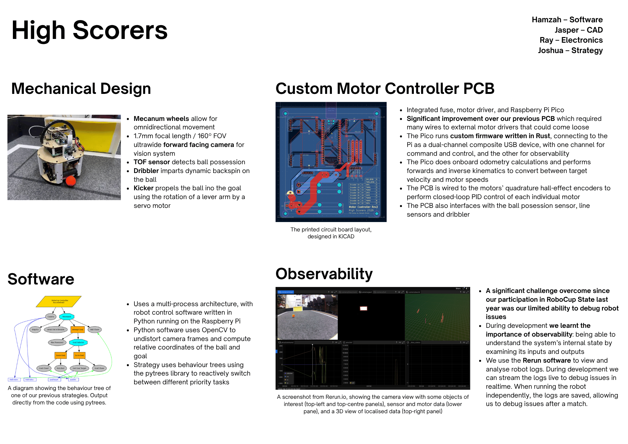This poster describes our overall robot design. My primary role was working on the control software, computer vision pipeline and PCB (printed circuit board) design but some other aspects of the robot are described here for context. Notably:

• Mecanum wheels allow the robot to move in any direction, moving in any combination of forwards, sideways or spinning in place. This allows the robot to quickly face the ball. This is similar to the omniwheel arrangement used by many other teams. We mainly chose mecanum wheels for their low cost.

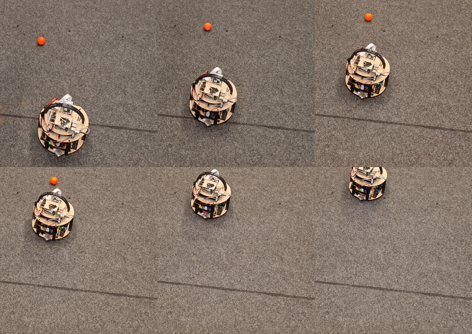
• The dribbler is a rotating drum designed to impart backspin on the ball. This dribbler, as well as the chassis was designed by another team member responsible for mechanical design. This way the robot can maintain possession of the ball. The dribbler drum is also driven by N20 motors from the same motor controller PCB, with the other side of the drum connected to a bearing. The 3D-printed drum has LEGO tires fitted over it for better grip. This is quite effective, as the robot can dribble the ball backwards to defend its goal: 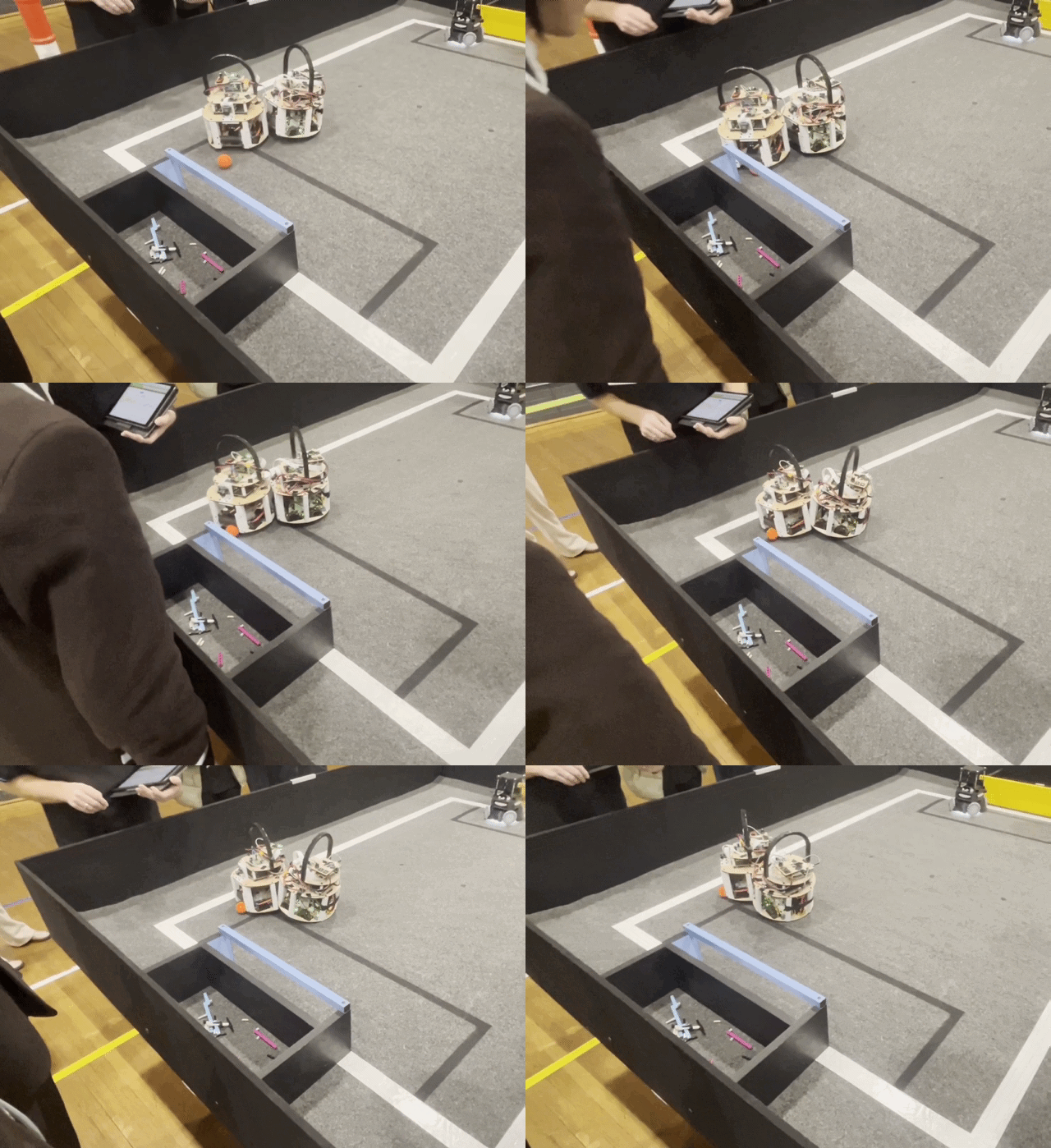No other team at the state competition had a dribbler, and the more effective and precise control of the ball enabled by it was a significant contributing factor to our success.

• The kicker mentioned on the poster was designed last-minute and had some interference issues with the dribbler so it had to be removed.

• When the robot possesses the ball it is out of view of the camera, so a VL53L0X time of flight (ToF) sensor allows the robot to ensure it really does have possession of the ball. When the ball enters the dribbler zone, it shortens the distance detected by the ToF sensor allowing the robot to register that it has successfully captured the ball. 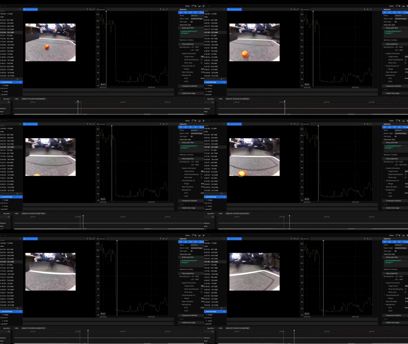The graph on the right in the above image shows the measurable decrease in distance measured by the sensor when the ball enters the dribbler.

PCB design

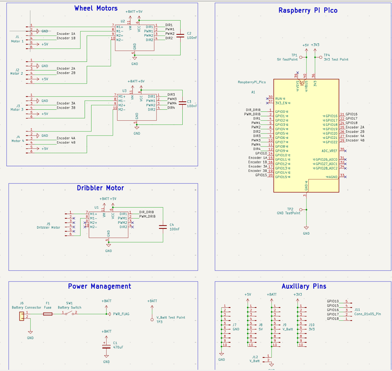
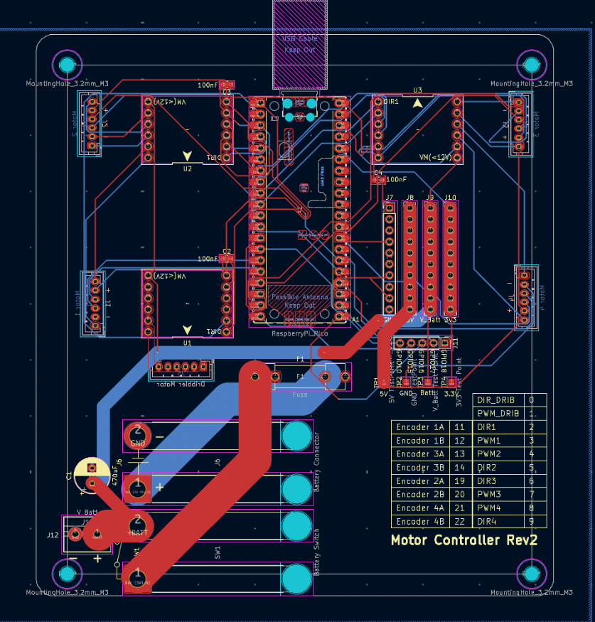
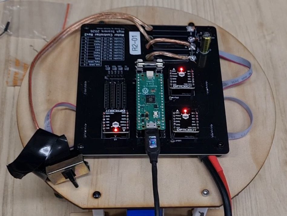
I designed the motor controller PCBs for these robots in KiCAD. These motor controller PCBs perform closed-loop motor control for the mecanum wheels, control the dribbler and distribute power from the battery with a fuse in case of short circuit.

Our robots use four individually controlled motors for the mecanum wheels which are connected to motor drivers (which each need 2 connections from the motor terminals to the driver, and PWM and direction connections from the driver to the MCU) and each of these motors have 4 further connections from the quadrature encoders reporting motor rotation to the MCU. That gives a total of 32 connections for locomotion alone.

Hence, the reasons I designed the PCBs were:

• To avoid needing to manually wire these connections during assembly, affording us the ability to rapidly assemble and disassemble portions of the robot to debug issues
• For consistency in pinout between the two robots
• For greater reliability: jumper wires can come loose or snap at joints if soldered

The first revision of this board as the first PCB I had ever designed, and the boards on our state competition robots were the second. To reduce the opportunity for error, this PCB uses breakout boards such as a Raspberry Pi Pico (a development board for the RP2040 MCU) and DRI0044 (a breakout for the TB6612FNG motor driver IC) boards which each hold those difficult-to-solder surface-mount ICs as well as their support circuitry.

These reliability improvements are a major theme of our team's work in 2026, and our success in the state competition was largely due to this: our robots worked more consistently, and when they were working they could quickly gain possession of the ball to easily score a goal.

Firmware

The Raspberry Pi Pico on the aforementioned PCB runs Rust firmware I wrote. This firmware takes movement commands from the main Raspberry Pi board over USB, determines motor speeds needed to achieve that movement, and performs closed loop control to keep motors at that speed. It uses the Embassy framework which provides a hardware abstraction layer and async runtime.

The diagram above describes the general architecture for the firmware. The kinematics and closed-loop control portions of this system are rather standard in mechatronic systems, however this level of closed-loop control is rare in RoboCup Junior. Recall that the robot has 3 axes of motion: longitudinal, lateral and yaw. Inverse kinematics takes a velocity for each of these 3 axes and converts it into appropriate mecanum wheel rotational velocities to achieve that chassis velocity. Forwards kinematics conversely takes the reported rotations from the motor encoder and converts it into a chassis velocity. The combination of these two allow us to make any planar movement on the robot.

The parts of the system I have described so far were already in place in the original MicroPython implementation I wrote in 2025. The reason I rewrote this firmware was related to the interface between the Raspberry Pi Pico (the microcontroller on our motor controller PCB) and the Raspberry Pi 4 (the main "brains" of the robot, processing camera data and making decisions). These two components are linked by a micro-USB cable, carrying power and data. Vanilla MicroPython does support taking input over USB (by sys.stdin or input) but this same serial channel is used for the MicroPython REPL and there is no native support for separating out serial channels or having any serious control over USB configuration. Overall this led to a more brittle system that was difficult to debug. I also made the mistake of trying to have odometry be reported asynchronously from velocity commands, but the MicroPython setup is really not designed for this in mind so I had lots of reliability issues.

Instead, in the Rust rewrite I created two separate USB communication device class (CDC) channels: one for debug logging and one synchronous request/response interface for sending commands. The Embassy embedded framework made this straightforward as I had complete control over USB packet processing on the device. In the diagram above you see COBS decode/encode blocks. COBS is a packet framing scheme (basically an encoding that allows both sides to know where commands start and end) so you may be wondering why a packet framing is needed when USB already involves sending packets. For simplicity, I chose to use USB CDC ACM (basically a serial interface) for the command channel, and this device class abstracts over the packets and rather represents data sent as a stream of bytes. Hence, a framing scheme is needed to delineate this stream.

The advantage of using CDC ACM is that on the Raspberry Pi side, the device appears as a pair of standard TTYs which can be read and written to with pyserial. In retrospect, I consider using CDC ACM to be a mistake. Alongside being conceptually inelegant, this scheme means data sent and received passes through the Linux kernel's TTY layer (which is highly non-deterministic) which has the right to buffer data arbitrarily. Despite my attempts to write resilient retry logic to resend commands if no response is seen, competition day exposed new link failure modes that our extensive testing could not find. If I were to build this interface again I would create a custom device class and write a user-space driver for it, to have greater visibility into hotplug and disconnect events.

Control software

Multi-process architecture

I wrote the control software that runs on Raspberry Pi OS. The architectural diagram below is from the repository README:

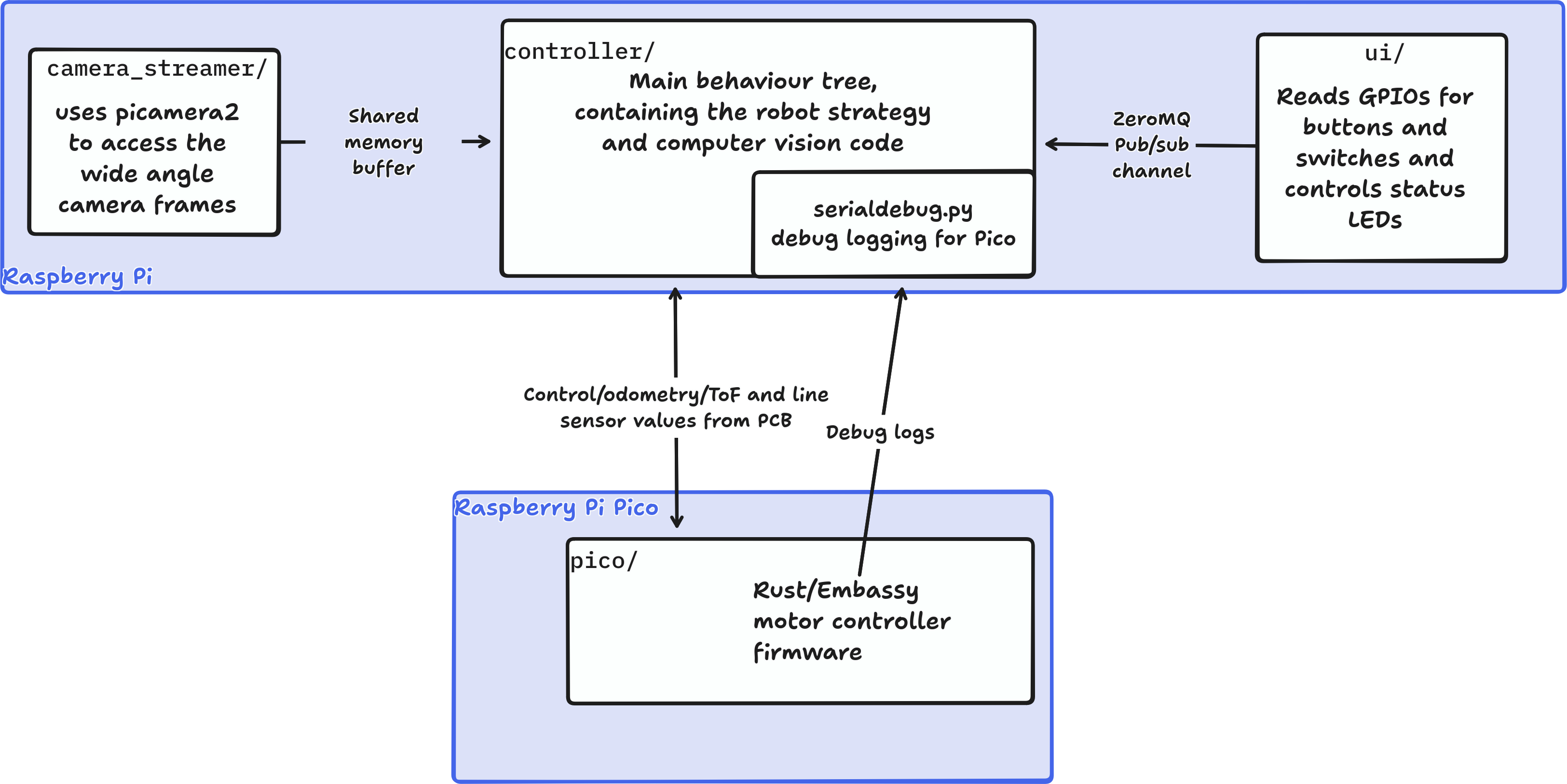
As shown, there are four different processes running in parallel:

• camera_streamer: This process accesses camera frames using the picamera2 library, writing them to a numpy array mapped in shared memory. I wrote it as a separate process because picamera2 is distributed by the Raspberry Pi OS package repositories and is dependent on shared libraries distributed that way. As I wanted to use virtual environments to manage dependencies for the controller process this had to be separated.

• controller: This is the main control process, sending commands to the motor controller board and reading in camera frames from camera_streamer. There is no synchronisation between camera_streamer and controller which means that there can be tearing artefacts if this process reads while the streamer is writing but this isn't an issue for our computer vision workloads. The robot strategy is organised in a behaviour tree using the pytrees library.

• serial_debug: This is a process spawned by the controller process to log data received through the USB debug channel to Rerun. This is primarily useful for troubleshooting motor encoders or tuning the PID loop.

• ui: This is kept separate from controller because of the need for the gpiozero library, which also poses problems when installed from a virtualenv. It handles button presses from the physical user interface on the robot (used for starting, stopping, changing goals, and powering down the robot) an publishes events over a ZeroMQ channel for the controller package to read. This process also controls two important status LEDs: a pulsing LED to show when the Raspberry Pi has completed boot, and another LED indicating which goal the robot is configured to score into.

camera_streamer, controller, and ui are all launched by their respective systemd units on boot. This also enables these processes to be restarted individually, and for their logs to be monitored using journalctl.

Behaviour tree

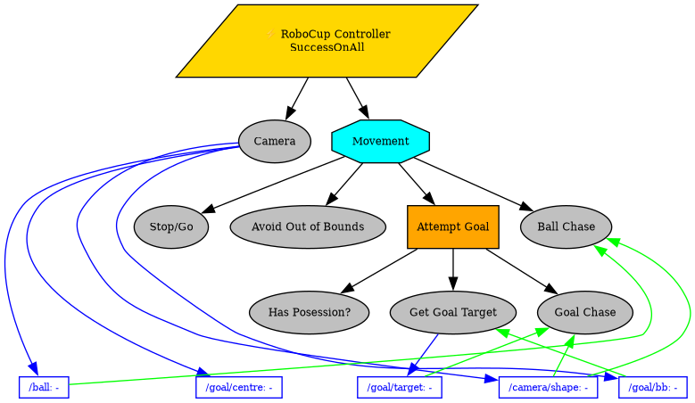
The behaviour tree is the decision making engine for our robots, and determines at a high level what the robot should do: for example whether the robot should move towards the goal or towards the ball. I chose behaviour trees over other approaches such as finite state machines mainly because they can very naturally represent a notion of cascading priorities, where a higher priority task (like gaining possession of the ball) can override a lower priority one (like searching for the ball).

In the above diagram, every node with black outline is a behaviour, which can briefly execute some code when they are "ticked". After being ticked, behaviours return RUNNING if the task they represent is ongoing or SUCCESS or FAILURE upon completion.

Behaviour trees have three main composites (these are nodes in the above diagram that point to multiple child nodes to combine their behaviours):

• Parallel (parallelogram in the above diagram): will tick every node under it every time it is ticked (overall effect of doing multiple tasks at once)
• Sequence (The rectangle in the diagram): each time it is ticked will tick each node under it in succession until any of its child nodes return RUNNING or FAILURE (overall effect of doing one task after another)
• Selector (The octagon in the diagram): each time it is ticked it will try each child node under it until any of its child nodes return RUNNING or SUCCESS (overall effect of trying different tasks until one of them works)

Despite the above behaviour tree being rather basic, it was reliable and this contributed to our robots' performance. In early stages of robotics development, high-level planning software is seldom a bottleneck, rather it is the hardware and low-level control software that determines a system's success. For almost all of our two year development, improving the reliability and performance of the lower levels of our stack was a better use of time than implementing a sophisticated strategy, because these strategies are contingent on reliable and effective hardware and control.

Computer vision and localisation

Our robots' camera setup is unconventional, as we use a wide-angle forward facing camera rather than a 360-degree mirror setup like most RoboCup Junior robots. The purpose of a RoboCup computer vision system is to identify the locations of the ball, goals and possibly field lines or even other robots. More sophisticated strategies become possible when robots can determine the physical relative coordinates of objects (in real-life units e.g. in millimetres), which is called localisation. Localisation is a prerequisite for proper trajectory planning and navigation, coordination between robots, and deduction of where the ball is (by Bayesian inference, for example).

I wrote our robots' computer vision system, and localisation by fusing camera data and odometry was my ultimate goal. However, as mentioned earlier, these more sophisticated techniques are contingent on having basic hardware functionality which I was also responsible for. In the time I had, I only implemented a partial localisation system which I will describe below. Localisation systems are really only seen at the international level in RoboCup Junior. The main alternative approach I have heard of relies on using LiDAR to locate the field walls. My approach is purely camera-based and not even requiring an additional mirror, thus bringing the potential to make localisation systems more accessible for less experienced teams.

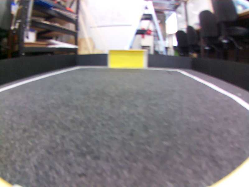This is an unprocessed camera frame from the wide angle camera. If you look at the white field lines, you will notice that they curve slightly due to a slight fisheye effect.

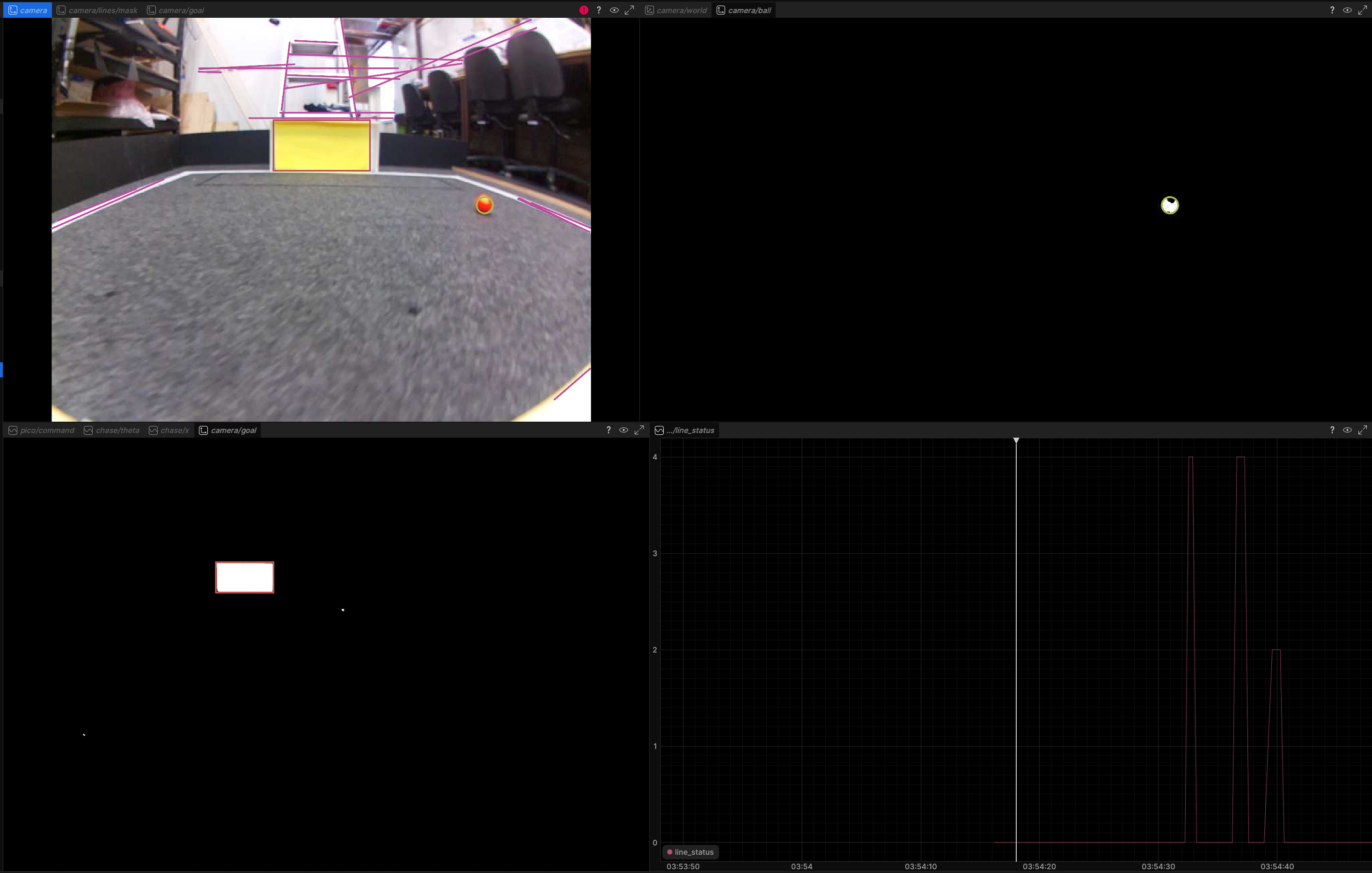On this raw frame, HSV colour thresholds are used to identify objects, since the RCJA soccer rules standardise the goals to be yellow and cyan, the ball to be orange and field lines to be white with particular dimensions. Some teams use more complex methods such as a machine learning model to do this, but I found simple colour thresholding to produce acceptable results at our stage of development. I also did further tuning after this screenshot is taken. The purple magenta lines drawn are detected by a sequence of white thresholding, canny edge detection, and then a probabilistic Hough line transform to detect field lines. At this step in the pipeline, you can see a lot of garbage lines detected above the field. These lines, alongside any other detections outside the field, will be filtered out in a later step of the process.

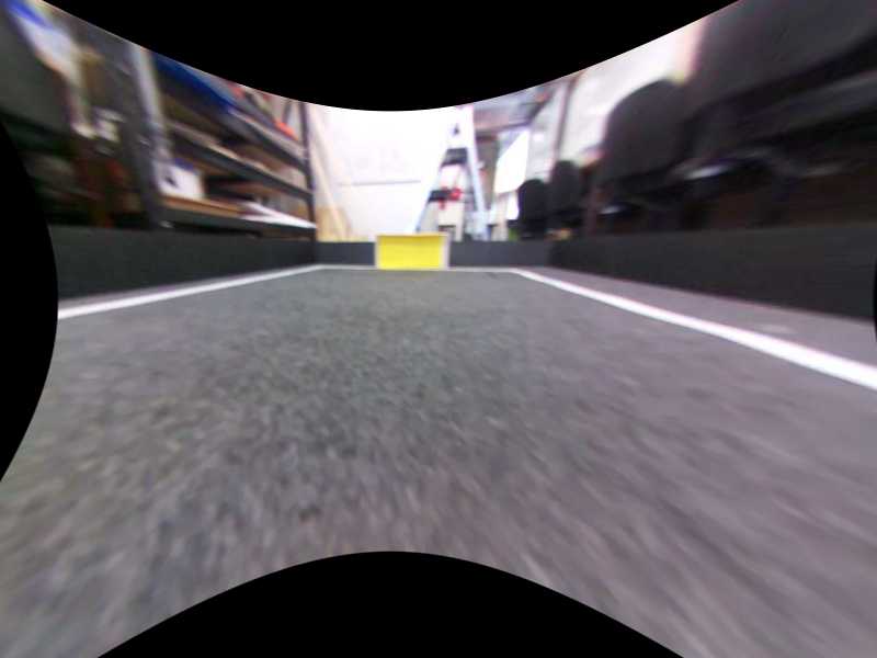
This is a view of the camera after undistortion. In controller/calibrate.py, a simple script calibrates the camera by fitting a model of fisheye distortion to the coordinates of a flat checkerboard pattern. The distortion coefficients, image resolution and camera matrix are written to a JSON file for later use. The undistorted image above was produced using these coefficients, and as you can see, the white lines are no longer curved as in the original image. Fully undistorting the image is very computationally expensive and is only done for debugging and visualisation purposes. Instead my code uses cv2.fisheye.undistortPoints to undistort only specific coordinates needed to be undistorted, as identified in the previous step. This undistortion step is required to be able to accurately determine real world coordinates of objects in the image.

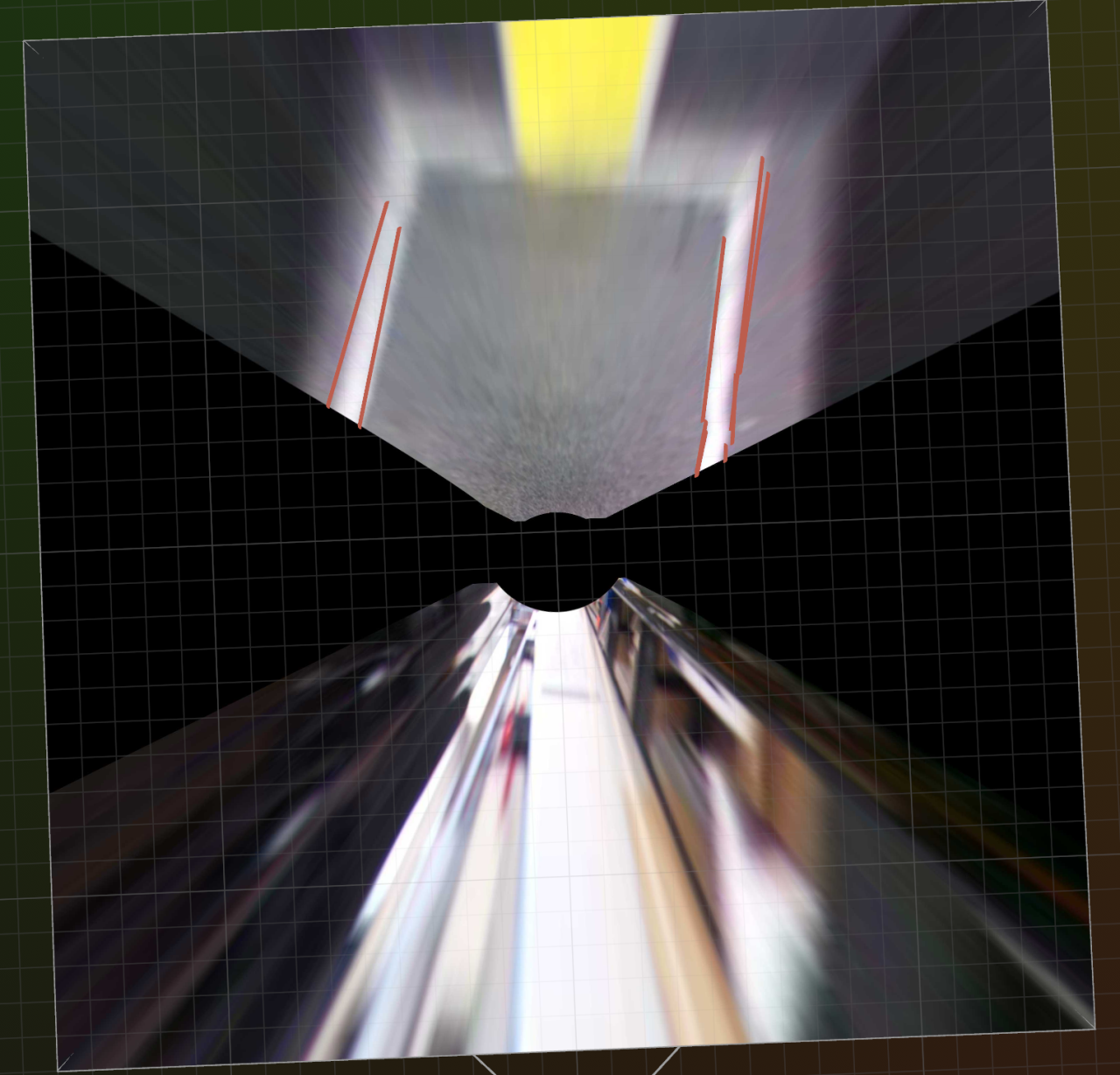
This is probably the most interesting step and is one that I have not ever seen in RoboCup Junior before. In this step, I project points on the field from the camera frame into real-world coordinates in millimetres, relative to the camera. This is effectively partial localisation, and in our control software this enables a much more effective ball acquisition tactic. I call this partial localisation because it can find the relative coordinates of any object on the field relative to the robot, but full localisation would give positions of objects in a shared coordinate frame relative to the field itself.

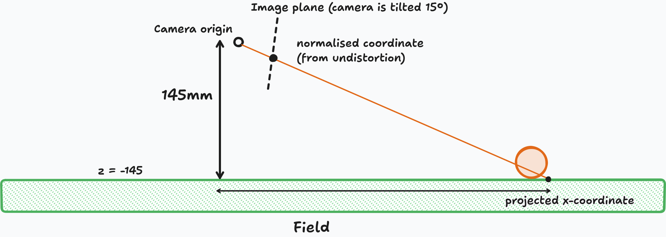
The above is a visualisation of all points being projected this way, but again the deployed code only projects the points that are needed for efficiency's sake. The principle that makes this projection possible is related to degrees of freedom. In the camera frame seen by a robot, a pixel has two degrees of freedom (row and column in image). For an object on the field, there are also two degrees of freedom (since the objects only move on the plane, they cannot be in the air). Thus, there is a mathematical function that transforms from one space to the other.

More specifically each pixel corresponds to a point on an image plane (an imaginary plane distance 1 away from the camera). cv2.fisheye.undistortPoints can give us coordinates on this plane. Draw a ray from the camera origin through this point on the image plane, extending it until it hits the field. The robot is a fixed height in millimetres above the field (the robot moves only in planar motion, it never travels up or down), so this intersection point between the field and this plane in the field can be easily found. Since the distance from the camera to the field is in millimetres, the coordinates of the intersection point on the field is also in millimetres. Thus, any object on the field that has been detected by the camera can be converted into coordinates on the field relative to the robot.

You may also notice a slight inaccuracy between the computed location between the projected coordinates of the ball and the real coordinates of the ball, as shown in the diagram. This could be compensated by using a z-plane offset by 21mm so the coordinates actually lie centered in the ball, but real-life testing found this inaccuracy to be negligible.

from scipy.spatial.transform import Rotation as R
rotation = R.from_euler("x", -CAMERA_ELEVATION_ANGLE)
ray = rotation.apply(ray)

Looking at the projection above, you will notice the large amount of garbage in the lower half of the image. This corresponds to the cases where the ray does not intersect with the field, meaning the object is above the horizon line. Mathematically this yields a computed location behind the camera, and the code that projects points individually discards those points. This image was produced by applying the homography matrix directly to the image which is why they are shown. Conveniently, this provides a reliable method to discard ball or goal detections outside the field.

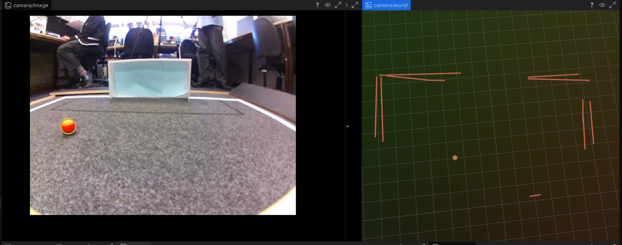
Thus, with only a single forward-facing camera, my algorithm can compute relative coordinates of any visible object on the field. In the time we had, I was only able to take advantage of this to better capture the ball, but as can be seen in the above image, the robot can get quite a lot of information about its field location based on this data.

This is a classic state estimation problem: sensor data provides incomplete and noisy data, and our goal is to infer the true state of the system. It was always my goal to implement an extended Kalman filter to fuse odometry and vision data to get good state estimates of robot positions and velocity. This would enable true localisation, which would enable far more sophisticated strategies. I studied this free online book to learn about these filters, written by the author of filterpy.

All bayesian filters operate around a loop of predict and measurement steps. IMU, odometry and velocity command data would be used during the predict steps to update the robot's state forward in time based on a motion of how these relate to the robot's state variables (position and velocity). Kalman filters keep track of error with a multivariate Gaussian distribution, and the error covariance grows during this step. Then, in the measurement step, data from field lines constitute absolute measurements of a robot's position. Different types of measurements can be made based on the type of 'feature' visible of field lines, for example seeing only two parallel field lines a given distance apart may provide a measurement of only the y and θ axes, while seeing a corner would update x, y and θ. Measurements can also incorporate uncertainties propagated from the vision system: for example a small segment of field line would propagate a greater uncertainty than a larger one.

Another useful application of filters that I wanted to implement was ball deduction. If the location of both robots is known, the ball not being visible actually conveys a large amount of information as to the location of the ball. A discrete bayesian filter breaks up the field into a number of rectangular 'cells', and assigns a probability of the ball being in that location. This is initially set to be a uniform probability distribution. Then, if the robot does not observe the ball in a cell, it can scale the probability for that cell down by a large factor (the probability remaining would be nonzero due to the uncertainty of measurement). This is the measure step. When the ball is seen, high probability can be assigned to those regions and a different state estimation technique such as a Kalman filter would be used instead. The update step is applying a convolution to the grid to propagate beliefs forward through time, as when time passes it becomes more uncertain whether those measurements in the past still apply.

This algorithm can quickly deduce where the ball is based on the area of the field that is visible (and the projection techniques mentioned earlier give us exactly this data), so the robot can effectively gain a sense of object permanence and infer things about the ball location even when it is not visible. It is a multi-hypothesis state estimation algorithm, making it suitable for this type of deduction as multiple possible locations for the ball can be considered.

This also gives rise to more complex defensive strategies. A popular RoboCup Junior strategy seen in international games is 'hiding the ball' where the ball is controlled by a dribbler to face an angle where it is not visible to other robots. This technique would defeat that, which is why we wanted to implement it. However, we did not see this technique in use at our state competition. Technically, the partial localisation data is enough to implement a 'hiding the ball' strategy, but I only achieved partial localisation a few days before the competition, and the ball acquisition improvements to follow were higher value per unit effort.

Ball acquisition tactic

The next problem is getting the robot to the ball, specifically such that it is within the possession of the dribbler. This is a control theory problem: I had to write some sort of controller that determines the appropriate command velocities for x (longitudinal movement), y (lateral movement) and θ (yaw rotation). In my initial implementation before partial localisation, I implemented it in the simplest way I could think of:

• If the ball is to the left, turn left
• If the ball is to the right turn right
• If the ball is within a central region in the image, go forwards
• If the ball is not visible spin in circles

The last step could be improved with the discrete Bayesian logic described above, but most of the time the ball is visible to at least one robot. Thus, improving how the robot gets to the ball when it is visible is the most useful part to optimise. Notice that the logic above takes no advantage of the lateral movement capability of the robot, so its path is necessarily more indirect.

Thinking about translational movement, the robot should always move in a vector towards the ball. Thus, the translational velocity should always be equal to the relative displacement of the ball (as determined by the projection algorithm described earlier) multiplied by some scalar. We want the robot to be aligned with the ball for it to enter the dribbler, so this is something a PID controller can do. At first glance, the translation also seems like something suitable for PID, however PID does exactly the opposite of what we want to do. PID control tries to get a system's state to a certain value and have it stay at that value, while we want to move towards the ball with some forwards velocity in order for it to be captured by the dribbler. Thus, the displacement vector approach to translation is the better approach. The code for this policy is rather simple:

theta = np.arctan2(target[0], target[1])

vel_theta = self.pid_theta(theta)

# assume vel_scale is a scalar constant for now
velocity = np.array([target[0], target[1]]) * vel_scale(theta)

# Clip velocity vector length to 300mm/s max
vel_length = np.linalg.norm(velocity)
if vel_length != 0:
    velocity *= min(vel_length, 300) / vel_length

# X-forwards coordinates
self.command.send_command(velocity[1], velocity[0], vel_theta, 1)

See the full code for the chase behaviour here.

In the days before the competition, I just hardcoded a constant translational velocity, and this policy was used through most of the competition (I was busy debugging hardware issues). This was generally successful at capturing the ball at long range, but when the robot started out close to the ball but misaligned, it would move towards the ball with not enough time to properly capture it in the dribbler.

So in the minutes before a match, I decided to fix it. The robot's speed should be a function of its alignment with the ball, with the speed being maximum when it is perfectly aligned, and zero when it is fully out of alignment (so that the robot has time to turn towards the ball). This reeks of \(y = 3\cos\theta\), however I thought this would not be 'aggressive' enough. The dribbler is quite wide, so I wanted to prefer speed over alignment slightly more than what that graph suggested. So I opened up Desmos and as a team we quickly found the parabola through those points. In retrospect I should have fitted a quartic, since this graph is only slightly more aggressive than cosine.

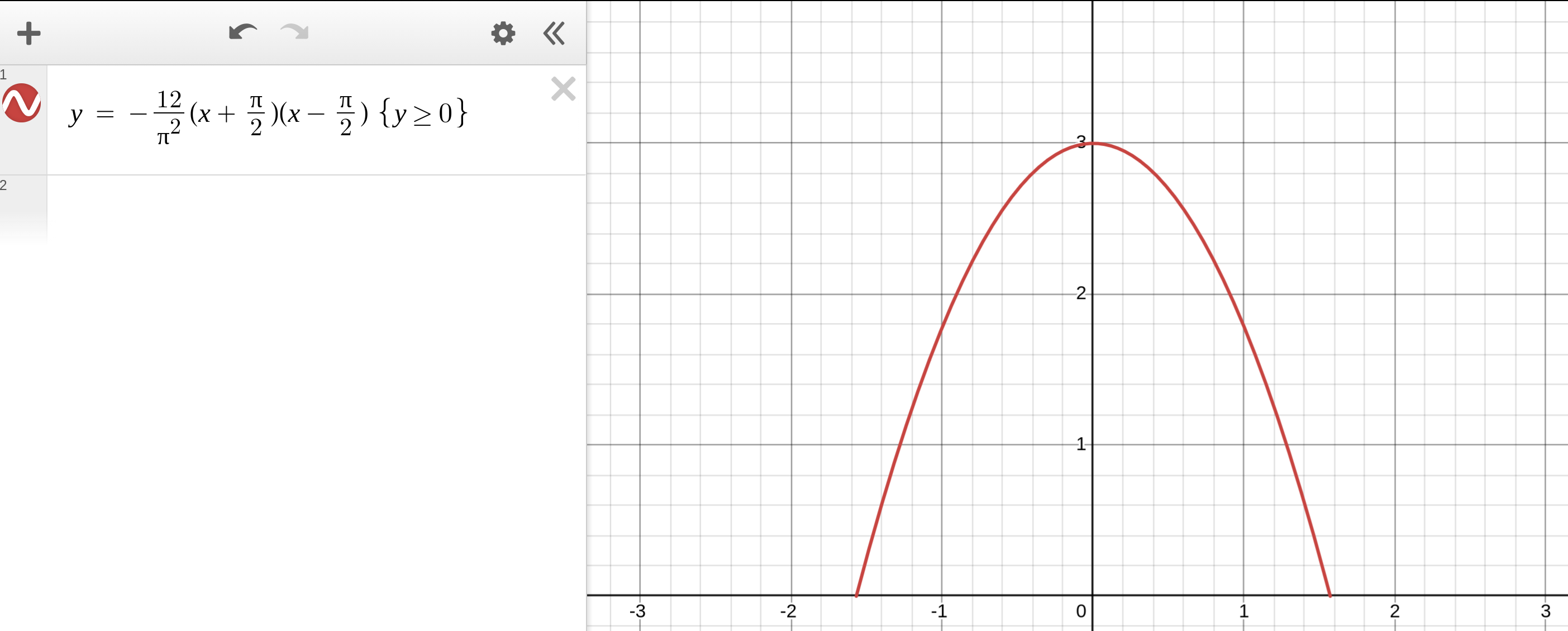
This improved the robots' ability to capture the ball at short range.

Open source release

Mechanical CAD, PCB designs and code are all released under open source licenses in our GitHub repository. I hope this can be of use for future teams.